Sentinel-1 product
Sentinel-1 product stage-in example.
Import the Python packages
[1]:
%matplotlib inline

import warnings
warnings.filterwarnings("ignore")
import os
import sys
import glob

import cioppy
ciop = cioppy.Cioppy()

import numpy as np
import matplotlib
import matplotlib.pyplot as plt
import matplotlib.colors as colors

from snappy import jpy
from snappy import ProductIO
from snappy import GPF
from snappy import HashMap

import gc

from shapely.wkt import loads

import folium
Search parameters
Set the catalogue endpoint to Sentinel-1:
[2]:
series = 'https://catalog.terradue.com/sentinel1/search'
Define the time of interest:
[3]:
start_date = '2017-09-01T00:00:00'
stop_date = '2017-12-10T23:59:59'
Define the area of interest:
[4]:
geom = 'MULTIPOLYGON (((26.832 9.5136, 28.6843 9.5136, 28.6843 7.8009, 26.832 7.8009, 26.832 9.5136)), ((32.0572 12.4549, 33.9087 12.4549, 33.9087 10.7344, 32.0572 10.7344, 32.0572 12.4549)), ((-5.5 17.26, -1.08 17.26, -1.08 13.5, -5.5 13.5, -5.5 17.26)), ((12.9415 13.7579, 14.6731 13.7579, 14.6731 12.0093, 12.9415 12.0093, 12.9415 13.7579)))'
Check the WKT validity:
[5]:
loads(geom)
[5]:

Build and submit the catalog search
[6]:
search_params = dict([('geom', geom),
                     ('start', start_date),
                     ('stop', stop_date),
                      ('do', 'terradue'),
                      ('pt', 'GRD')])
[7]:
search = ciop.search(end_point = series,
                     params = search_params,
                     output_fields='self,enclosure,identifier,wkt',
                     model='GeoTime')
[8]:
discovery_locations = []

for index, elem in enumerate(search):
    discovery_locations.append([t[::-1] for t in list(loads(elem['wkt']).exterior.coords)])

    print(index, elem['identifier'])
(0, 'S1A_IW_GRDH_1SDV_20171210T182114_20171210T182139_019644_021603_0AB1')
(1, 'S1A_IW_GRDH_1SDV_20171210T182049_20171210T182114_019644_021603_96BE')
(2, 'S1A_IW_GRDH_1SDV_20171210T182024_20171210T182049_019644_021603_0A33')
(3, 'S1A_IW_GRDH_1SDV_20171210T181959_20171210T182024_019644_021603_D3D2')
(4, 'S1A_IW_GRDH_1SDV_20171209T033328_20171209T033353_019620_02154C_F3B6')
(5, 'S1A_IW_GRDH_1SDV_20171209T033259_20171209T033328_019620_02154C_8F85')
(6, 'S1A_IW_GRDH_1SDV_20171208T183711_20171208T183736_019615_02151E_1BB2')
(7, 'S1A_IW_GRDH_1SDV_20171208T183646_20171208T183711_019615_02151E_561D')
(8, 'S1A_IW_GRDH_1SDV_20171208T183621_20171208T183646_019615_02151E_6721')
(9, 'S1B_IW_GRDH_1SDV_20171208T034043_20171208T034108_008622_00F4FA_EBD2')
(10, 'S1B_IW_GRDH_1SDV_20171208T034018_20171208T034043_008622_00F4FA_796B')
(11, 'S1A_IW_GRDH_1SDV_20171207T035045_20171207T035110_019591_021463_A5A3')
(12, 'S1A_IW_GRDH_1SDV_20171207T035016_20171207T035045_019591_021463_0026')
(13, 'S1A_IW_GRDH_1SDV_20171206T171418_20171206T171443_019585_021433_D800')
(14, 'S1A_IW_GRDH_1SDV_20171206T171353_20171206T171418_019585_021433_5C1A')
(15, 'S1B_IW_GRDH_1SDV_20171206T035811_20171206T035836_008593_00F41C_389F')
(16, 'S1B_IW_GRDH_1SDV_20171206T035746_20171206T035811_008593_00F41C_DC3A')
(17, 'S1B_IW_GRDH_1SDV_20171206T035721_20171206T035746_008593_00F41C_3E3C')
(18, 'S1A_IW_GRDH_1SDV_20171205T181306_20171205T181331_019571_0213C3_1B7E')
(19, 'S1A_IW_GRDH_1SDV_20171205T181241_20171205T181306_019571_0213C3_00F4')
Plot the AOIs and the search results
[9]:
aois = []

for index, aoi in enumerate(loads(geom)):

    aois.append(np.asarray([t[::-1] for t in list(aoi.exterior.coords)]).tolist())
[10]:
s1_index = 5
[11]:
lat = (loads(geom).bounds[3]+loads(geom).bounds[1])/2
lon = (loads(geom).bounds[2]+loads(geom).bounds[0])/2

zoom_start = 4

m = folium.Map(location=[lat, lon], zoom_start=zoom_start)

radius = 4
folium.CircleMarker(
    location=[lat, lon],
    radius=radius,
    color='#FF0000',
    stroke=False,
    fill=True,
    fill_opacity=0.6,
    opacity=1,
    popup='{} pixels'.format(radius),
    tooltip='I am in pixels',
).add_to(m)

folium.PolyLine(
    locations=aois,
    color='#FF0000',
    weight=2,
    tooltip='Japan flooding',
).add_to(m)

folium.PolyLine(
    locations=discovery_locations,
    color='orange',
    weight=1,
    opacity=1,
    smooth_factor=0,
).add_to(m)

folium.PolyLine(
    locations=[t[::-1] for t in list(loads(search[s1_index]['wkt']).exterior.coords)],
    color='green',
    weight=1,
    opacity=1,
    smooth_factor=0,
).add_to(m)

folium.PolyLine(
    locations=aois[1],
    color='green',
    weight=1,
    opacity=1,
    smooth_factor=0,
).add_to(m)

map_path = os.path.join(os.sep, 'workspace', 'tmp', 'maps')

if not os.path.isdir(map_path):
    os.makedirs(map_path)

m.save(os.path.join(map_path,'map.html'))

m
[11]:
[12]:
s1_identifier = search[s1_index]['identifier']
s1_reference = search[s1_index]['self']
Prepare the variables assignment for the Jupyter Notebook streaming executable
[13]:
print 'input_identifier = \'%s\'' % s1_identifier
input_identifier = 'S1A_IW_GRDH_1SDV_20171209T033259_20171209T033328_019620_02154C_8F85'
[14]:
print 'input_reference = \'%s\'' % s1_reference
input_reference = 'https://catalog.terradue.com/sentinel1/search?format=atom&uid=S1A_IW_GRDH_1SDV_20171209T033259_20171209T033328_019620_02154C_8F85'
Stage-in the data
Define the local folder where to stage-in the data to:
[15]:
data_path = os.path.join(os.sep, 'workspace', 'tmp', 'data')
[16]:
if not os.path.isdir(data_path):
    os.makedirs(data_path)
[17]:
try:
    retrieved = ciop.copy(search[s1_index]['enclosure'], data_path)
except:
    retrieved = os.path.join(data_path, search[s1_index]['identifier'])
Plot a subset
[18]:
s1meta = "manifest.safe"
s1prd = os.path.join(data_path, s1_identifier, s1_identifier + '.SAFE', s1meta)

s1prd
[18]:
'/workspace/tmp/data/S1A_IW_GRDH_1SDV_20171209T033259_20171209T033328_019620_02154C_8F85/S1A_IW_GRDH_1SDV_20171209T033259_20171209T033328_019620_02154C_8F85.SAFE/manifest.safe'
[19]:
x = 13727
y = 10438
width = 6186
height = 6942

reader = ProductIO.getProductReader("SENTINEL-1")
product = reader.readProductNodes(s1prd, None)

HashMap = jpy.get_type('java.util.HashMap')
GPF.getDefaultInstance().getOperatorSpiRegistry().loadOperatorSpis()

parameters = HashMap()
parameters.put('copyMetadata', True)
parameters.put('region', "%s,%s,%s,%s" % (x, y, width, height))
subset = GPF.createProduct('Subset', parameters, product)

product = None
gc.collect()
[19]:
101
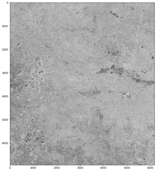
[20]:
%matplotlib inline

def plotBand(product, band, vmin, vmax):

    band = product.getBand(band)

    w = band.getRasterWidth()
    h = band.getRasterHeight()

    band_data = np.zeros(w * h, np.float32)
    band.readPixels(0, 0, w, h, band_data)

    band_data.shape = h, w

    width = 12
    height = 12
    plt.figure(figsize=(width, height))
    imgplot = plt.imshow(band_data, cmap=plt.cm.binary, vmin=vmin, vmax=vmax)

    return imgplot

plotBand(subset, 'Amplitude_VV', 0, 350)
[20]:
<matplotlib.image.AxesImage at 0x7f4f9f6f0310>
[21]:
subset = None
gc.collect()
[21]:
0